Chaos!

In day to day use, the word "Chaos" has some negative meanings, such as disorder, messiness etc. However, mathematically, the study of chaos is in fact extremely beautiful and endlessly fascinating. Fractals are the pictures of chaos theory. While we often tend to think of chaos as referring to disorder, chaos theory really deals with the transitions between order and disorder.

We will explore a few natural systems that often show chaotic behavior. Under some circumstances, they may behave predictably, and then at surprising times they may change in radically unpredictable ways. Two of the most commonly studied systems in chaos theory are population ecology, and weather prediction.

We will begin with an exploration of population ecology, which can be modeled with a simple equation. Amazingly, the equation that describes how the numbers of predators and prey can oscillate (fluctuate up and down) - also generates the Mandelbrot Set!

Rabbits and Coyotes

Let us begin by exploring the population of animals in an ecosystem. The graph below shows one possible oscillating relationship between the number of rabbits and the number of coyotes. This regular fluctuation makes intuitive sense, because when there are lots of rabbits (coyote food), then in a little while there will be a boom in the population of coyotes. After a while they will drive down the number of rabbits; after that, the number of coyotes will drop, as their food supply is scarce, and then the rabbit population will rebound and the cycle begins again. We will see that this regular oscillation is not the only way this system can work however. Sometimes there can be unpredictable population explosions or collapses, and the length of time between the cycles can also change unpredictably.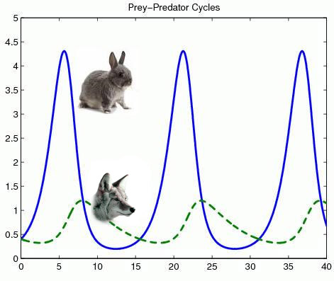

The population of rabbits and coyotes sometimes alternates in a regular, predictable fashion.

If we start with a given number of rabbits, call it P₀ (for initial population). The Verhulst Equation was developed in the 19th century to predict the number of rabbits in the following generation. Of course, rabbits don't live in isolation, they have limited resources to eat, and they also have predators that eat them, such as coyotes. We can iterate the equation to determine the population at the next generation, and then take that value and plug it back into the equation to find the population of the next generation and so on. The equation looks like:

P_n+1 = P_n + CP_n(1-P_n/K)

Ok, what does this mean? Let's start simply. We're interested in the population at the next generation, which we call P_n+1. Well, we need to add the current population to the number of new rabbits born, so that is why we add the term P_n to the equation. Next we'll address the fertility of rabbits. This is the factor 'C' in the equation. The number of new rabbits - in the absence of predators, or food limits - equals the number of rabbits P_n times the fertility factor C. If C = 2, for example, there would be twice as many rabbits created. So if none of the rabbits died, there would then be:
P₁ = P₀ + 2P₀ = 3P₀ rabbits. We can iterate the equation again to find the population of the next generation, which would be:
P₂ = P₁ + 2P₁
And if we plug in the value of P₁ we can find that:
P₂ = 3P₀ + 6P₀ = 9P₀
This is called Exponential Growth. and the population will get very large, very quickly.

Clearly there is more to the picture than this. The rabbits will run out of food, so we need to introduce another factor in the equation to make it more realistic. This is the value 'K', which is called the carrying capacity of the environment, and it provides an upper limit on the growth of the population. So we introduce the term (1-P/K). K is the maximum number of animals the ecosystem can sustain. When P/K is small, that is when the population is much less than the carrying capacity, the term (1-P/K) is almost 1, which means it has little effect on the growth, so the population starts off growing exponentially.

However, when the population P approaches the carrying capacity K, then P/K approaches 1, and the term (1-P/K) approaches 0. The Verhulst equation then tells us that the population will gradually stop growing as it plateaus at the maximum sustainable value. Or, the population may overshoot the carrying capacity, and then decline in the following generation to a sustainable level.

The graph below shows the exponential growth model in red and the growth model that converges to the carrying capacity in blue.

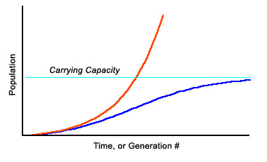An unconstrained population growth model (red) grows exponentially. A constrained growth model (blue)
starts similarly but is tempered by the (1-P/K) term and follows a sigmoid curve up to a plateau.

Start with 100 fish in a pond (P₀). Assume a fertility factor of .5, and that the carrying capacity of the pond is 200.
Use the Verhulst equation to calculate the number of fish at the next generation, P₁: [ ]
Calculate the number at the second generation, P₂: [ ]
Hint: your answer should be larger than the carrying capacity, which is unsustainable. At the next iteration, the term CP₂(1-P₂/K) will be negative, bringing the population back down again.
What is the population P₃ at the third generation? [ ]

We will explore the behavior of the Verhulst equation in more detail as it relates to population, but before we do that let's see what sort of fractal it creates.

The equation P_n+1 = P_n + CP_n(1-P_n/K) can be multplied out to be expressed as:
P_n+1 = P_n + CP_n + CP_n²/K
Recall from the lesson on Mandelbrot Universality, that when you iterate an equation that has a squaring function in it (or even approximates one), in the complex plane, you will find Mandelbrot Sets. Since this equation contains the term P_n², it should not be surprising that we can easily find Mandelbrot Sets in the fractal below. Zoom into and explore this closely related fractal known as the Lambda fractal.

The lambda fractal, a close relative of the Mandelbrot Set. Click mouse to Zoom In <Ctrl>-Click mouse to Zoom Out

To describe the ecological system more completely with predators and prey, we would create an equation that models the population of coyotes and link it to the equation for the rabbits.

However, we don't need to do this to discover chaotic behavior. Given the right conditions,the population of a single species can fluctuate chaotically, as we will see in the next section.